General considerations about wide-field imaging

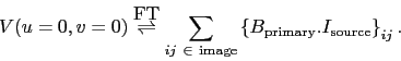
The measurement equation for a millimeter interferometer is to a good approximation (after calibration)

$$V(u,v) = \mbox{FT}\ensuremath{\displaystyle\left\{ B_\ensur... ...thrm{primary}}.I_\ensuremath{\mathrm{source}} \right\}}(u,v)+N$$ (5.1)

where $\mbox{FT}\ensuremath{\displaystyle\left\{ F \right\}}(f)$ is the bi-dimensional Fourier transform of the function $F$ taken at the spatial frequency $f$, $I_\ensuremath{\mathrm{source}}$ the sky intensity, $B_\ensuremath{\mathrm{primary}}$ the primary beam of the interferometer (i.e. a Gaussian of FWHM the natural resolution of the single-dish antenna composing the interferometer), $N$ some thermal noise and $V(u,v)$ the calibrated visibility at the spatial frequency $u,v$. The product of the sky intensity by the primary beam, which ``quickly'' decreases to zero, implies that an interferometer looking at a particular direction of the sky will have its field-of-view limited by the size of the primary beam.

To image a field-of-view larger than the primary beam size, the antennae of an interferometer will be successively pointed in different directions of the sky typically separated by half the size of the primary beam. This process is called mosaicing and the result requires specific imaging and deconvolution steps. Another possibility is to acquire data as the interferometer antenna continuously slew through a portion of the sky. This second observing mode is called interferometric On-The-Fly (OTF). While mosaicing is standard at PdBI (see section 5.2), some efforts are currently done to commission the OTF observing mode.

Mosaicing and OTF clearly belongs to wide-field imaging. However considerations about wide-field imaging start as soon as the size of the source is larger than about 1/3 to 1/2 of the interferometer primary beam. Indeed, a multiplicative interferometer (e.g. all interferometer in the (sub)mm range) is a bandpass instrument, i.e. it filters not only the large spatial frequencies (this is the effect of the finite resolution of the instrument) but also the small spatial frequencies (all the frequencies smaller than typically the diameter of the interferometer antennas). An important consequence is that a multiplicative interferometer do not measure the total flux of the observed source. This derives immediately from the following property of the Fourier Transform: The Fourier transform of a function evaluated at zero spacial frequency is equal to the integral of your function. Adapting this to our notation, this gives

$$V(u=0,v=0) \stackrel{\mbox{FT}}{\rightleftharpoons} \sum_{i... ...athrm{primary}}.I_\ensuremath{\mathrm{source}} \right\}}_{ij}.$$ (5.2)

i.e. the visibility at the center of the $uv$ plane is the total intensity of the source. As a multiplicative interferometer filters out in particular $V(u=0,v=0)$, the information about the total flux of the observed source is lost. In summary, a multiplicative interferometer only gives information about the way the flux of the source is distributed in the spatial frequencies larger than the primary beam but no information about the total flux.

Deconvolution algorithms use, in one way or another, the information of the flux at the smallest measured spatial frequencies to extrapolate the total flux of the source. This works correctly when the size of the source is small compared to the primary beam of the interferometer. The extreme case is a point source at the phase center for which the amplitude of all the visibilities is constant and equal to the total flux of the source: Extrapolation is then exact. However, the larger the size of the source, the worst the extrapolation, which then underestimates the total source flux. This is the well-known problem of the missing flux that observers sometimes note when comparing the flux of the source delivered by a mm interferometer with the flux observed with a single-dish antenna. The transition between right and wrong extrapolation is not well documented. It depends on the repartition of the flux with spatial frequencies but also of the signal-to-noise ratio of the measured spatial frequencies. It is often agreed that the transition happens for sizes between 1/3 and 1/2 of the interferometer primary beam. For larger source size, information from a single-dish telescope is needed to fill in the missing information and to thus obtain a correct result. This is the object of section 5.3.