Observing strategy

A bolometer measures other contributions (e.g. the atmospheric emission), which usually domintes the measured signal. Moreover, MAMBO bolometers have a finite time response. The strategy to map a source must take care of both effects. One way is to wobble the secondary in the scanning direction. We note that it is customary to scan in the azimuthal direction because this allows to scan at nearly constant airmass (i.e. at constant elevation). However, when mapping an elongated source (e.g. an edge-on galaxy disk), the restoration algorithms work best when scanning along the smallest source size. In addition, the observing mode (wobbling) introduces strong boundary conditions, which in general implies that the whole array must scan over the full source size. In addition, a portion of blanked sky (typically 3 times the full width at half maximum of the telescope beam) must be be observed to baseline the data.

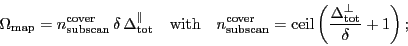
In summary, if the PI wants to map a source of size $\ensuremath{\Delta^\ensuremath{\mathrm{\Vert}}_\ensuremath{\mathrm{sou}}}\times \ensuremath{\Delta^\ensuremath{\mathrm{\bot}}_\ensuremath{\mathrm{sou}}}$, the total scanned size will have to be $\ensuremath{\Delta^\ensuremath{\mathrm{\Vert}}_\ensuremath{\mathrm{tot}}}\times \ensuremath{\Delta^\ensuremath{\mathrm{\bot}}_\ensuremath{\mathrm{tot}}}$ with

$$\ensuremath{\Delta^\ensuremath{\mathrm{\bot}}_\ensuremath{\mathrm{tot}}} = \ensuremath{\Delta^\ensuremath{\mathrm{\bot}}_\ensuremath{\mathrm{sou}}},$$ (10)

$$\ensuremath{\Delta^\ensuremath{\mathrm{\Vert}}_\ensuremath{\mathrm{tot}}} = \ensuremath{\Delta^\ensuremath{\mathrm{\Vert}}_\ensuremath{\mathr... ...hrow}}}+ \ensuremath{\Delta^\ensuremath{\mathrm{}}_\ensuremath{\mathrm{base}}},$$ (11)

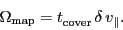
where is the linear array size, is the wobbler throw and is the size of blanked sky used for baselining. The rows of the map (i.e. the subscans) are scanned at constant velocity, . The size of the row will be . Each row will be an independent subscan of duration . The separation between two rows will be . If the area to be mapped is called , the time to cover it once is called and the number of subscans per coverage is called , the following relationships hold

$$\ensuremath{\Omega_\ensuremath{\mathrm{map}}}= \ensuremath{... ..._\ensuremath{\mathrm{tot}}}}{\ensuremath{\delta}}+1 \right) };$$ (12)

$$\ensuremath{\Delta^\ensuremath{\mathrm{\Vert}}_\ensuremath{... ...emath{t^\ensuremath{\mathrm{}}_\ensuremath{\mathrm{subscan}}};$$ (13)

$$\ensuremath{\Omega_\ensuremath{\mathrm{map}}}= \ensuremath{... ...nsuremath{\delta}\,\ensuremath{v_\ensuremath{\mathrm{\Vert}}}.$$ (14)

Note that the grouping of the subscans in coverages is independent of the grouping of the subscans in scans, e.g. the same scan can finish a coverage of the source and start a new one.